EXOFAST - HAT-P-3b example

This will walk you through various examples using public data of HAT-P-3b. This fit is generally more difficult than most fits because the RV data are sparse, and so not very constraining. That makes this a useful demonstration of the types of problems that you may encounter (and what you can do about it), but try not to be intimidated -- it's usually much easier.

Presumably, you have your own data files. If you're missing RVs of a known planets, you can usually get them from the Exoplanet Archive (for HAT-P-3b, both the light curve and RVs can be found here. While you can do the fit with just transit data or just RV data, you can learn much more about the system with both (and that's the real advantage of EXOFAST).

The light curves and RV files at NStED have no standard, and are typically not in the required format. The RVs must be in three columns: BJD_TDB, RV (m/s) and error (m/s). The light curves must have at least 3 columns: BJD_TDB, normalized flux (mean out of transit flux approximately equals 1), and error. Optionally, it can have any number of additional columns, which will be used to detrend the light curve (e.g., airmass at each time). We have converted the files to this format, which you can download (RV and transit).

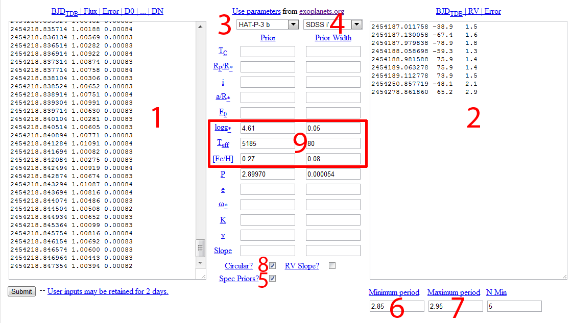
Paste them into the appropriate forms (marked #1 and #2 below), select the planet from the drop down menu (#3; HAT-P-3 b) and the band the transit data were taken in (#4; SDSS i'), and check the box "Spec priors?" (#5) -- this tells it to grab the spectroscopic priors from exoplanets.org for logg, Teff, and [Fe/H].

It'll also get the starting values for the transit from exoplanets.org, to make the fitting more robust (otherwise it'll use Hot-Jupiter-like guesses, which is usually good enough). Now click submit.

First, it finds the period with a Lomb-Scargle periodogram of the RV data. Assuming a circular orbit, it finds the "N min" best periods. Normally, there will be one obvious period, and it'll just work. This time, however, you'll notice that there are 4 periods with low χ²_ν:

Best peaks in the RV fit:
     T_C            Period        ecosw        esinw        K          gamma          slope      chi^2      chi^2/dof
2454194.513285     2.509754    -0.040753     0.013526   115.808745   -22.060623     0.000000    73.595057    24.531686
2454196.563903     3.190485    -0.214598    -0.016286   111.215690   -10.738981     0.000000     5.837212     1.945737
2454195.676539     2.900505    -0.129177     0.013844   104.960806   -16.348920     0.000000    10.519117     3.506372
2454195.934438     2.988335    -0.157248    -0.047552   106.561277   -14.253449     0.000000     4.929913     1.643304
2454195.150633     2.728094    -0.062298     0.056450   101.638085   -19.409819     0.000000     6.324167     2.108056

It will proceed with the best fit (lowest χ²_ν of the RV data, in this case a period of 2.99 days) but that doesn't mean that's correct. In fact, a good indication that it's NOT correct are the χ² of the combined fits:

Combined fit:
Chi^2 of Transit data = 1500.3209 (368 data points)
Chi^2 of RV data = 4649.3067 (9 data points)
Chi^2 of Priors = 19.175438 (3 priors)
Chi^2/dof = 16.812228

Then, if you look at the best-fit parameters and models, you'll see it's not a good fit at all. The eccentricity is really high, the RV data don't fit at all, and the planet actually orbits inside the star (creating some strange light curve models). This is really an indication that the best fit transit and best fit RV were not consistent, and thus the 2.99 day period is likely the problem.

We can force it to pick the next most likely (3.19 days) instead. Go back and insert 3.15 as the minimum period and 3.25 as the maximum period (#6 and #7), which will only allow the 3.19 day peak and submit. This works, but you should be leary for two reasons. First, you should investigate the other two periods, because they looked equally likely. Second, you'll see from the RV plot that the orbit really only has data at 3 or 4 distinct phases, and so it doesn't really have the power to constrain the eccentricity (i.e., it's probably just fitting the noise). We should investigate options for a circular orbit, noting the χ² values for the combined fit. Note that these are after the errors have been scaled to force P(χ²) = 0.5 for the individual fits.

When we look the four best periods, we find:

Chi^2/dof = 16.812228 (P = 2.99 days)
Chi^2/dof = 1.0227054 (P = 3.19 days)
Chi^2/dof = 1.0750580 (P = 2.65 days)
Chi^2/dof = 1.0062160 (P = 2.90 days)

So it looks like the 2.9 day period is slightly favored, but there's really no telling between 2.65, 2.90, and 3.19 days (note that the RV only preferred period of 2.72 days was changed to 2.65 days in the combined fit). Since we really don't have the power to contrain the eccentricity, we'll fix it to zero by checking the circular box (#8), and try again:

Best peaks in the RV fit:
     T_C            Period        ecosw        esinw        K          gamma          slope      chi^2      chi^2/dof
      1.107424     2.509629     0.000000     0.000000   111.702373   -19.695690     0.000000    79.680061    15.936012
      0.032483     3.191384     0.000000     0.000000    88.122421    -8.571517     0.000000    60.684224    12.136845
      1.241369     2.901193     0.000000     0.000000    90.201515   -14.637107     0.000000    31.508634     6.301727
      0.604251     2.985977     0.000000     0.000000    89.044937   -12.943334     0.000000    34.917544     6.983509
      1.105912     2.727992     0.000000     0.000000    95.094301   -17.178435     0.000000    27.056734     5.411347
Chi^2/dof = 5.4113468
Scaling errors by 2.4935620

We see the same periods, though the 3.19 day period is much less appealing. Let's look at all of them anyway:

Chi^2/dof = 1.0431960 (P = 2.65 days)
Chi^2/dof = 0.99045819 (P = 2.90 days the combined fit finds this minimum for both 2.99 and 2.90 days)
Chi^2/dof = 1.0015210 (P = 3.19 days)

The 2.5 day period one failed altogether, with a very poor fit to the RV data and this error:

EXOFAST_GETMCMCSCALE: Parameter 6 is unconstrained. Check your starting conditions

This essentially means the transit time predicted from the RVs were so far off that all the transit models were flat lines. We can safely ignore this period.

So still, there's a slight preference for the 2.90 day period, but two others (2.65 and 3.19 days) are reasonable. We really need more information to be sure. Fortunately (as will almost always be the case), we know the period precisely from the transit survey (2.89970 +/- 0.000054 days), so we know which to use. We can also use that value as an explicit prior by entering it in the prior and width boxes (note, however, that the period prior and the limits on the Lomb-Scargle periodogram are independent. You need to make sure you have the right period for both.

Not in exoplanets.org

So what happens if your planet is not in exoplanets.org (like a new planet)? In this case, we'll pretend we can't select the planet. So go back and deselect HAT-P-3b, reset the period ranges, and uncheck the "Spec priors?" and "Circular?" boxes. Now it won't use any information from exoplanets.org to start the fit, nor will it get the spectroscopic priors on logg, Teff, or [Fe/H].

In order to use the information from both RV and Transit data sets, we'll need our own priors on Teff and [Fe/H] (logg helps, but is adequately constrained by the transit + Torres relations alone). These can all be estimated from a precise spectrum. If we don't have that, Teff can be estimated from multi-color photometry and we can assume the metalicity is solar. In this example, we'll just grab the values from exoplanets.org manually (Teff = 5190 +/- 80, [Fe/H] = 0.27 +/- 0.08), and pretend we measured them from somewhere. Insert those values into the appropriate "prior" and "prior width" boxes. If you don't have these priors, enter roughly solar values with very large error bars (Teff = 6000 +/- 2000, [Fe/H] = 0 +/- 1), and then do not believe the stellar parameters or anything derived from them. However, be warned that since a transit alone can determine the stellar density, the stellar parameters can make a difference to the actual light curve model. If you get a high contribution to the χ² from the priors, you may want to revisit them.

Now we get a different error:

Best peaks in the RV fit:
     T_C            Period        ecosw        esinw        K          gamma          slope      chi^2      chi^2/dof
2454194.513285     2.509754    -0.040753     0.013526   115.808745   -22.060623     0.000000    73.595057    24.531686
2454196.563903     3.190485    -0.214598    -0.016286   111.215690   -10.738981     0.000000     5.837212     1.945737
2454195.676539     2.900505    -0.129177     0.013844   104.960806   -16.348920     0.000000    10.519117     3.506372
2454195.934438     2.988335    -0.157248    -0.047552   106.561277   -14.253449     0.000000     4.929913     1.643304
2454195.150633     2.728094    -0.062298     0.056450   101.638085   -19.409819     0.000000     6.324167     2.108056
Chi^2/dof = 1.6433043
Scaling errors by 1.4434929

Transit fit:
Chi^2/dof = 63.478024
Scaling errors by 7.9746943

ERROR: Transit fit not constrained. Check your starting conditions.

This error basically means the same thing as the previous one. Because we didn't use the values from exoplanets.org to start the transit fit, it only relied on the RV to predict the transit time. Since the period it picked was wrong, the predicted transit time was way off, and all transit models it tried were indistinguishable, flat lines.

Now we can play the same game, narrowing the window of periods allowed by the Lomb-Scargle periodogram, trying circular and eccentric fits, and we'll end up with roughly the same results as when we used the values from exoplanets.org.

RV data only

Since not every planet transits, often times, all you'll have is RV data. Leave the transit textarea blank. While it's not necessary to fit, you are required to plug in logg, Teff, and [Fe/H]. It'll use the Torres relation to derive a stellar mass and radius, which is used, along with the RV parameters, to derive a bunch of interesting things about the system, including transit probabilities, durations, and times. For the transit durations, it assumes a point planet (Rp=0) and a central crossing (b=0). Just like above, you'll have to explore different periods that seem nearly equally likely (and with/without eccentricity), but you won't have any additional data (e.g., the transit time) as a sanity check. If you were really trying to fit a data set this messy with the RV alone, you'd just need more data.

Transit data only

This is the least robust because the transit model depends on the eccentricity, argument of periastron, and period, which a single transit alone can't constrain very well. Fortunately, this shouldn't be necessary for the vast majority of planets. If at all possible, try to find a source of RVs from the literature. If they don't exist (such as for faint Kepler data), proceed.

In principle, the period can be constrained if mulitple transits are given, but deriving it from first principles requires a Box Least Squares algorithm, which we don't do. If you have specified a planet name and checked the "Spec Priors?" box, and your data span less than one period, it will automatically grab the period and period width from exoplanets.org. Otherwise, you'll need to give it a starting value for the period, even if it's determined from the same photometry you're fitting. If you have multiple transits, a prior width on the period is not necessary, otherwise, the results may not be believable. Failing to include a prior width may cause the period to wander dramatically, and many things scale with the period, so none of your fits will be believable. A warning is issued if this is attempted.

Forcing the orbit to be circular (by checking the "Circular?" box) is highly recommended for most transit-only fits. If the orbit is eccentric, you probably know that from RVs, so you should include them instead of a prior. Nevertheless, if you'd prefer, you can include a prior on eccentricity and the argument of periastron if the orbit is eccentric.

Like the combined fit, we require you to provide an estimate of Teff and [Fe/H] so we can derive the stellar properties and therefore the planetary properties.